METHODS

Tail Musculature Reconstruction

The tail muscles of Kentrosaurus were reconstructed using the terminology employed in Carpenter et al. (2005). As in Arbour (2009), extant crocodylians were chosen as a guide, because crocodylians are the sole extant archosaurs with long and muscular tails.

Muscle paths of Alligator and other extant tailed reptiles were taken from the literature (Romer 1923a, 1927; Gasc 1981; Frey et al. 1989; Cong et al. 1998) and dissection data. On the basis of these reports, combined with muscle reconstructions of closely related taxa (Coombs 1979; Carpenter et al. 2005; Arbour 2009) and other dinosaurs (e.g., Romer 1923b), the major tail muscles of Kentrosaurus were reconstructed in cross section at the base of the tail immediately distal to the cloaca and at roughly one-third the tail length (Figure 1). These two points were chosen because the force produced in the basal part of the tail influences tail swing speeds the most, and because the size of the vertebrae, which correlates with that of the soft parts, decreases almost linearly along the tail, so that distal parts can be modeled by scaling down the anterior parts. In order to determine muscle diameters, the cross section photographs of the alligator tail were imported into McNeel Associates Rhinoceros 4.0 NURBS Modeling for Window©, and the muscle and bone outlines traced. Surfaces were created to fill in the muscle outlines, so that the cross section areas as well as area centroids could be directly calculated in Rhinoceros 4.0. Because data from dissection and from the cross section photographs disagrees with the common practice to limit soft tissues to the extent of the bones (tips of transverse processes, neural spines, haemapophyses as in, e.g., Paul 1987; Christiansen 1996; Carpenter et al. 2005; Arbour 2009) three versions were created. The first (henceforth 'slim'; Figure 4.1) follows the literature and assumes that the soft tissues form an ellipse with the tips of the neural arch and the haemapophysis determining the long axis, and the tips of the transverse processes forming the short axis. The second model ('croc'; Figure 4.2) has axes proportionally as much longer than the extent of the bone as the average values of the measurements taken on the alligator cross section photographs. However, the model is not proportionally equivalent to the alligator, but has somewhat smaller muscle cross section areas, because the alligator's muscles bulge out, while those of the model do not. This model conforms roughly to the general extent of the tail muscles in extant reptiles as determined by dissection by Persons (2009) and via digital 3D reconstruction based on CT data by Allen et al. (2009).The third model ('medium'; Figure 4.3) has an elliptical shape like the 'slim' model, but axes lengths are the arithmetic average of the 'slim' and 'croc' models. The alligator section used for the muscle reconstruction at the base of the tail is shown in Figure 4.4, the tracing of it in Figure 4.5, combined with a muscle reconstruction for the alligator following the dinosaur muscle reconstruction paradigm (elliptical model). Mm. ischiocaudalis and iliocaudalis were not separated in the tracings and reconstructions, because their contact line in the Alligator cross sections is often difficult to determine exactly. Their exact sizes relative to each other are not of importance for the models computed here. Also, at the very base of the tail of the alligator, a part of the m. iliocaudalis runs between the transverse process and the m. caudofemoralis, which was here counted as part of the m. caudofemoralis to achieve consistency with the reconstructions from the literature. For comparison, tracings of the reconstructions of Stegosaurus in Carpenter et al. (2005) and the slim and the muscular version for ankylosaurs in Arbour (2009) are shown in Figure 4.6-4.8, scaled to the same vertebral size.

The torque values T each muscle could produce were calculated based on these reconstructions:

(1),

with A being the cross section area, P the specific tension, and l the moment arm of the muscle. The moment arms were determined by measuring the horizontal distance of the area centroids of the muscles from the sagittal plane in the CAD program. Values for specific tension vary widely in the literature, from as low as 15 N/cm² to as high as 100 N/cm² (e.g., Fick 1911; Franke and Bethe 1919; Barmé 1964; Langenberg 1970; Maganaris et al. 2001). Carpenter et al. (2005) use two values to bracket the probable range, 39 N/cm² and 78 N/cm², based on data in Ikai and Fukunaga (1968). Arbour (2009) used 20 N/cm², based on studies on humans and cats. A detailed study on the m. quadriceps group in humans found values between 50 N/cm²and 60 N/cm² (O'Brien et al. 2010). Marx et al. (2006) report values between 25 N/cm² to 45 N/cm² from a wide size range of animals, including values of ~ 35 N/cm² from a rhinoceros.

At the top end of the spread reported in the literature, values over 70 N/cm² stem mainly from older literature and can be discounted because of methodological problems. The remaining variation of values is partly explained by various physical, methodological and biological reasons (Bottinelli and Reggiani 2000). Also, the joint angles at which the measurements of moment arms are made strongly influence the estimated specific tension (Winter and Challis 2003). Force production of a muscle depends also on the speed of the contraction, with slow continuous contraction allowing higher values than rapid contraction (Alexander et al. 1999). Since tail swinging involves relatively slow contractions, the values of 20 N/cm²and 50 N/cm² are used here, as they bracket the most likely range. 39 N/cm² and 78 N/cm² are used to create comparability to Carpenter et al. (2005). The former value is close enough to the middle of the 20-50 N/cm² range that results using it can be regarded as the likely upper end of the best estimate range. Table 1 lists the muscle cross section areas and torques for the reconstructions at the base of the tail.

This method for estimating available torques is a gross simplification, ignoring important details such as the internal structure of the muscles (straight-fibered or pinnate, which determines if there is a difference between geometrical and physiological muscle cross section) or the complex relationship between muscle fiber length, muscle contraction, and force production. Highly detailed musculoskeletal modeling in a dedicated program (e.g., SIMM, see Delp and Loan [1995, 2000]; Hutchinson et al. [2005]) could take these and other factors into account, but the gain in accuracy may well be negated by the inaccuracies necessarily included in the estimates of muscle mass, motion range, spike position, and angle and specific tension. A detailed sensitivity analysis covering all these factors is beyond the scope of this work.

CAD Model Creation

The high-detail 3D model was created in Rhinoceros 4.0® on the basis of NURBS ellipsoids, which were deformed via control point (node) editing. Spikes and plates were created as separate elements (Figure 5.1-5.4). Of the tail three additional versions were created (Figure 5.5) corresponding to the three muscle cross section models.

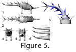
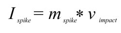
The limbs of the model were sectioned into functional units (e.g., brachium, antebrachium, manus). In the neck, trunk, and tail, one segment should ideally correspond to one vertebra plus soft tissues, as is the case for the initial, detailed model of the tail (Figure 5.5), but this would lead to such a high number of individual bodies to be handled by the CAE program that calculation times would become intolerable. Therefore, a simpler sectioning of the 'slim' tail model was created, dividing the tail into five parts, with the spikes distributed following Janensch (1925), and incorporated into the respective sections (Figure 5.1-5.4). These sections do not correspond to specific points in the tail (changes in morphology of the caudal vertebrae or in mobility), because the changes in vertebral shape are continuous, and mobility between vertebrae remains constant (Mallison 2010a). The number of segments is a compromise, attempting to keep computing times tolerable (each additional segment doubles computing time) while using a sufficient number of segments to achieve overall similarity between the geometry of the real tail's motion and that of the model. Figure 5.6 shows both the detailed and simplified tail models in a strongly laterally deflected pose in comparison.

Instead of creating similar simplified versions for the 'medium' and 'croc' tail models, the density of the simple model was accordingly increased in the CAE software.

The trunk was split into two parts, one for the sacral region, one for the rest, and the neck was arbitrarily split into five sections.

NASTRAN Modeling

Computer Aided Engineering (CAE) was conducted in MSC.visualNASTRAN 4D© by MSC Corp. and NX 5.0© by Siemens AG. The CAD model parts were imported as *.stl (binary ASCII polygon mesh) files. Because the sole physical property of significance for the simulations presented here is density, all other values such as thermal conductivity, specific heat, and yield stresses were set to the defaults (i.e., those of steel). Mass was adjusted as appropriate by setting a specific density for each individual object, as described below.

Some simulations were conducted by defining joint motions through table or formula input, based on desired results (e.g., orientation per time for a swing across the full arc). Henceforth, these are termed 'prescribed motion' models. They can result in motions that are impossible, e.g., because the required accelerations could not be produced by the available musculature, or because the motion range was exceeded. Therefore, internal (through data derived within the simulation) and external (through comparison to motion range analysis (Mallison 2010a) or further calculations outside NASTRAN) controls were necessary and are described where appropriate. Other models limited the motion range of joints in the CAE program a priori to the values determined by the range of motion analysis by Mallison (2010a). On the basis of the determined maximum muscle forces and moment arms, joint torques were calculated and used to drive these models, here termed 'torque' models.

Most of the 'prescribed motion' models could be simulated with simple Euler integration, but all 'torque' models required the more detailed and accurate Kutta-Merson integration with variable time steps. The mathematical basics of both methods are described in Fox (1962). Because of the much higher calculation time demands of Kutta-Merson integration, only a limited number of models could be computed.

The detailed tail models with 32 segments, and thus 33 joints (31 between segments, one to anchor the tail to the hip, and one to connect the spikes; Figure 5.5), cannot be computed as 'torque' models, because the required accuracy would result in calculation times upwards of a week per model run. Therefore, the simplified tail version with only five segments was used instead (Figure 5.1, 5.5). This model does not result in an identical overall curvature, but the moment arms are sufficiently similar that it can be used instead of the more detailed tail model, because the uncertainties in all other respect (muscle reconstruction, range of motion analysis, implicit assumptions in the 3D CAD model, flexion rates of the tail) have a much larger influence on the accuracy of results. The slight inertia differences between the two tail models do not play a significant role.

Mass Estimates and COM Position

Variations of the density of all parts of the CAD model were undertaken, to simulate larger or smaller amounts of soft tissues than those assumed in the three CAD models. The position of the center of mass (COM) was determined in the CAE program.

The fraction of total body weight supported by each pair of limbs is identical to 1 minus the limb pair's proportional distance from the COM (Alexander 1989; see also Henderson 2006). Changes in an animal's posture alter the moment arms of body parts, shifting the position of the overall COM. This change can be tracked in NASTRAN, as well as the lateral accelerations of the entire animal, here measured at the posterior body segment. These tests were run with both the simplified and the detailed tail models.

Several models of tail swings were run with the tail tip impacting a large generic object representing a mid-sized or large predator, to test the effect of impacts on the inertia of the entire animal. The impacts were set to a coefficient of restitution of 0.5, meaning that 50% of the total impact energy is transferred back to the tail, while the other half is consumed in tissue deformation. This value is probably too high and underestimates the stability of the animal.

Continuous Tail Swings

Tail motions were modeled first as 'prescribed motion' models, with continuous accelerations and decelerations in each joint (i.e., the entire tail musculature was assumed to be actively involved in creating the swing), using a simple sinusoid function with a 1 s, 1.5 s and a 2 s period. Crocodiles and alligators as well as large monitor lizards can all move their tail through large arcs in between below 0.3 s for smaller animals and less than 0.5 s for large animals (> 3m body length, pers. obs.), although it is unclear whether these motions involve the full motion range or the maximum possible speed. Flexion per joint was set to 2.5°, 5°, and 6°, with all joints given equal values, because mobility along the tail apparently was constant (Mallison 2010a). Greater values would lead to the tail tip spike hitting the trunk, unless the tail was in an extended position. The required torque at the base of the tail and the speed of the tail tip in relation to the deflection angle were measured. Additionally, the models were adjusted to achieve the same overall swing times to cover the whole arc, but distribute the applied torque values more evenly. All these models were run without any target for the tail to impact on. This way, it could be determined if a strike missing the target would unbalance the animal.

Whiplash Tail Swings

A sinusoid deflection rate leads to maximum speed at the half-angle (i.e., when the tail is straight). Whiplash actions shift the maximum speed angle and can increase the top speed significantly. Since the mechanics of whiplashes are complex, no attempt was made to calculate ideal motions to create maximum speed or a certain high speed across as large an arc as possible. Rather, simple motions were improved by trial and error. When results showed speeds high enough to cause serious injury to other animals, optimization of the motion was halted.

The high speeds involved in the 'crack' of a bullwhip rely on two basic properties: flexibility and a tapering diameter from the base to the tip (Bernstein et al. 1958). Whip dynamics are described in detail for the tails of diplodocid dinosaurs in Myhrvold and Currie (1997). In principle, to create high speeds at the end of the whip, a wave running down the length of the whip is created by suddenly halting or reversing rotation at the base. The wave gains speed on its way because the constant angular momentum is applied to ever decreasing amounts of mass under an ever shortening radius. The simplest way to create such a motion in the tail of Kentrosaurus with a maximum of angular momentum was acceleration of the base of the tail, which acts as the whip handle, starting at maximal lateroflexion and continuing through the entire motion arc, with the osteological or soft tissue stops halting motion suddenly when maximum lateroflexion on the opposing side is achieved. Then, the base of the tail is accelerated in the opposite direction, here using two-thirds of the maximum calculated torque. The more distal joints were similarly accelerated for appropriate intervals into the direction of the swing using the full calculated torque, and then accelerated in the opposing direction using two-thirds of the maximum torque (i.e., as in the continuous swing models the entire tail was assumed to be actively contributing to the motion). Depending on when exactly which joint's direction was reversed, the top speed varied widely, and the point at which the tail tip achieved this speed was located in different places. No attempts were made to maximize the speeds, or the arc across which it was achieved, but a roughly exponential increase in tail tip speed through the motion was aimed for. Similar motion patterns were observed in alligators, both through direct observation and on videos, when the animals used their tails to strike at objects.

Several different versions of the whipping motion models were created, with shorter or longer 'handles', but since those with the shortest handle produce the highest speeds resembled the observed motions of extant crocodylians the most, and are osteologically feasible, only these motions are discussed here. Whiplash motions were modeled only as 'torque' models, using the simplified 5-segment version of the tail. Whiplash motions were also modeled without impacts on target, to determine if the stability of the pose was influenced by strikes missing the target.

Impact Forces

The pressure created by a spike impact on another animal depends on the mass and speed of the spike, which determine the impulse transferred, and on the stopping time, as well as the contact area. The impulse delivered to the target is

(2),

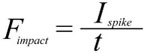
and the maximum force exerted

(3).

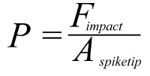
Applied over a target area A this force creates a pressure P

(4),

where I_spike is the impulse of the spike, m_spike its mass, and v_impact its velocity at the time of impact, F_impact the force it can deliver, t the stopping time, and A_spiketip the area of the spike tip that contacts the target.

For the sake of simplicity, the area of the spike tip is here assumed to be identical to that calculated for tail spikes of Stegosaurus by Carpenter et al. (2005), 0.28 cm², for penetrating strikes. Stopping time is difficult to estimate, and Carpenter et al. (2005) and Arbour (2009) use the conservative value of 0.33 s. Another example of high-energy collisions from the paleontological literature is head-butting behavior in pachycephalosaurs (Snively and Cox 2008). From the deceleration distances and speeds given in that publication, the implicitly assumed stopping time can be calculated, which varies between 0.018 s and 0.11 s for the average deceleration distance. However, these deceleration distances include not only the skull-skull collision, but additionally assume neck and potentially hindlimb motions (Snively and Cox 2008). For investigating a collision between a Kentrosaurus tail spike and, e.g., the skull or torso of a large theropod, it is impossible to estimate whether, and how, the target body would move or deform. However, data is available for a collision involving a relatively stiff element, somewhat similar to a tail spike, and a softer, deformable object, which can represent a bone/soft tissue complex: Tsaousidis and Zatsiorsky (1996) and Tol et al. (2002) give the time a football player's foot is in contact with the ball at around 0.016 s. Since force is inversely proportional to stopping time, using 0.016 s instead of 0.333 s as the stopping time means a ~21-fold increase in force, and thus pressure. Even shorter contact times of roughly 0.01 s are reported for football collisions in Australian rules football by Ball (2008), slightly higher values by Smith et al. (2009), who report an average of 0.022 s. What value should reasonably be used for calculating a tail-antagonist collision? Pachycephalosaurs appear to be adapted to cushioning impacts by flexion of the vertebral column (Carpenter 1997, figure 1), which are taken into account by Snively and Cox (2008), whereas a tail strike against a predator's flank could not be thus or similarly absorbed. Also, one must assume that in agonistic behavior, the participants have time to preposition their bodies and pretense muscles to maximize stopping time, while a predator probably did not have this chance when a stegosaur defended itself by tail strikes.

In bighorn sheep, deceleration takes place in less than 0.3 s (Kitchener 1988), again in a situation where there are shock-absorbing structures present that extend the stopping time (Farke 2008). Therefore, significantly shorter stopping times for the bone–bone collisions (spike with thin horn cover against skull, ribs, limbs near joints) investigated here appear reasonable, and 0.05 s is arbitrarily selected as the sole tested value. This value is close to the average determined from Snively and Cox (2008), and thus probably too long, resulting in an underestimation of the impact forces at least for strikes hitting bone. Longer stopping times would certainly be created by collision with large amounts of soft tissue, but such tissues have much lower resistance to shear stress, so that comparable injuries would result.